Monte Carlo simulation
What is a Monte Carlo simulation?
A Monte Carlo simulation is a mathematical technique that simulates the range of possible outcomes for an uncertain event. These predictions are based on an estimated range of values instead of a fixed set of values and evolve randomly. Computers use Monte Carlo simulations to analyze data and predict a future outcome based on a course of action.
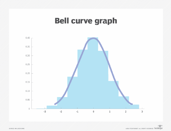
First, Monte Carlo simulations use a probability distribution for any variable that has inherent uncertainty. Then, it recalculates the results many times, using a different set of random numbers within the estimated range each time. This process generates many probable outcomes, which become more accurate as the number of inputs grows. In other words, the different outcomes form a normal distribution or bell curve, where the most common outcome is in the middle of the curve.

The Monte Carlo method has been described as "faking it a billion times until the reality emerges." It relies on the assumption that many random samples mimic patterns in the total population.
Importance of Monte Carlo simulations
Monte Carlo simulations are simple conceptually but enable users to solve problems in complex systems. They are particularly useful for long-term predictions because of their accuracy. Monte Carlo simulations are also a good alternative to machine learning when there isn't enough data to make a machine learning model accurate. As the number of inputs increases, so does the number of forecasts.
They also enable accurate simulations involving randomness. For a simple example, someone could use a Monte Carlo simulation to calculate the probability of a particular outcome -- say, rolling a seven -- when rolling two dice. There are 36 possible combinations, and six of those combinations add up to seven. The mathematical or expected probability of rolling a seven is 6/36, or 16.67%.
External factors, such as the shape of the dice or the surface they are rolled on, cause the actual or experimental probability to be different from the mathematical probability. Rolling the dice 1,000 times and getting a seven on 170 of those times would be the actual probability -- 170/1,000, or 17%, which is close to the actual probability but not exact. Each roll would be an iteration of the Monte Carlo simulation, which gets more accurate with each iteration. This property -- that the actual probability gets closer to the exact probability with more iterations -- is known as the law of large numbers.
Someone could use Microsoft Excel, IBM SPSS Statistics or a similar program to run this experiment.
The 4 steps in a Monte Carlo simulation
Although they might vary from case to case, the general steps to a Monte Carlo simulation are as follows:
- Build the model. Determine the mathematical model or transfer algorithm.
- Choose the variables to simulate. Pick the variables, and determine an appropriate probability distribution for each random variable.
- Run repeated simulations. Run the random variables through the mathematical model to perform many iterations of the simulation.
- Aggregate the results, and determine the mean, standard deviation and variant to determine if the result is as expected. Visualize the results on a histogram.
Monte Carlo simulation use cases
Monte Carlo simulations can be used for a spectrum of different industries. Finance is one of the most common use case examples, but any industry that involves predicting an inherently uncertain condition has a use for it.
Industry use cases for a Monte Carlo simulation include the following:
- Finance, such as risk assessment and long-term forecasting.
- Project management, such as estimating the duration or cost of a project.
- Engineering and physics, such as analyzing weather patterns, traffic flow or energy distribution.
- Quality control and testing, such as estimating the reliability and failure rate of a product.
- Healthcare and biomedicine, such as modeling the spread of diseases.
Use cases for Monte Carlo simulations also encompass different technologies. In IT alone, there a many use cases for Monte Carlo simulations. Some of those use cases specific to IT are the following:
- Network and system design. Monte Carlo simulations can be used to model different designs, identify potential bottlenecks, and perform capacity planning and resource allocation.
- Artificial intelligence. Monte Carlo simulations provide the basis for resampling techniques for estimating the accuracy of a model on a given data set.
- Cybersecurity. Monte Carlo simulations can be used to simulate different cyber attacks, evaluate the probability of them occurring, evaluate their hypothetical impact and identify vulnerabilities in IT systems.
- Performance testing. Monte Carlo simulations can be used for load testing applications and estimating the potential impact for increased usage or scaling.
Monte Carlo simulations are used in research and real-world business applications. They are specifically useful in research because of their ability to uncover data insights and enable the researcher to see multiple possible outcomes. Real-world scenarios for Monte Carlo simulations include the following:
- A researcher performing a risk assessment of potential toxic chemicals in South Korean cabbage kimchi.
- A telecom service provider gauging the ability of its network to handle swells in viewer traffic during the Olympics.
- A company tracking potential price movements of a given asset to price stock options.
- A random walk study of the spread of COVID-19.
- A smartphone manufacturer measuring a smartphone's performance in different temperatures.
- An analyst predicting the outcomes of a presidential election.
Advantages of Monte Carlo simulations
Monte Carlo simulations are used in many different areas for a reason. They are a relatively simple way to make complex predictions. They offer answers to hypothetical questions and assign a certain level of order to randomness. Other advantages of Monte Carlo simulations include the following:
- Improve decision-making. Monte Carlo simulations help users make decisions with a degree of confidence.
- Solve complex problems simply. Monte Carlo simulations show both what could happen and how likely each outcome is
- Visualize the range of possible outcomes and their likelihood of occurring. Monte Carlo simulations make it easy to visualize what the result of a standard decision or outcome might be next to the result of an unusual outcome.
Drawbacks of Monte Carlo simulations
Despite the advantages of Monte Carlo simulations, there are disadvantages. Like any simulation, it uses historical data for a future projection, which carries the risk of being inaccurate. Specific drawbacks of Monte Carlo simulations include the following:
- Processing power. Monte Carlo simulations require many iterations to be accurate. Running many iterations takes time and energy and can be computationally intensive.
- Input bias. This can be damaging if the data used for input is inaccurate or incomplete.
- Sensitivity to the chosen probability distribution. It is important to choose an appropriate probability distribution for the problem. Choosing the wrong one can render the results meaningless.
Common probability distributions used in Monte Carlo simulations
Probability distributions represent a range of values between two limits and can consist of discrete or continuous values. Discrete probability distributions are plotted as a sequence of finite numbers in a table, whereas continuous distributions are plotted as a curve between two points on a graph.
Some common probability distributions in Monte Carlo simulations are the following:
- Normal distributions. These are continuous distributions where the most data points cluster toward the middle. It is also called a bell curve or Gaussian distribution.
- Triangular distributions. These are continuous distributions with fixed minimum and maximum values. They can be either symmetrical, where the most probable value equals the mean and the median, or asymmetrical.
- Uniform distributions. These are continuous distributions by known minimum and maximum values. All outcomes have the same probability of occurring.
- Lognormal distributions. These are continuous distributions by mean and standard deviation. The values are positive and create a curve that skews right.
![Graphic of different probability distributions]()
Different probability distributions have different shapes and are suitable for different contexts. - Exponential distributions. These continuous distributions are used to illustrate the time between independent occurrences given the occurrence rate.
- Weibull distributions. These continuous distributions can model skewed data and approximate other distributions.
- Poisson distributions. These discrete probability distributions describe the probability of an event occurring in X periods of time.
- Discrete distributions. These discrete probability distributions help define the finite values of all possible outcome values.
Monte Carlo simulations can be implemented in programming languages. To implement a few common distributions in Python, use the following code:
- Normal distribution: numpy.random.normal.
- Triangular distribution: numpy.random.triangular.
- Uniform distribution: numpy.random.uniform.
- Weibull distribution: numpy.random.weibull.
History of the Monte Carlo simulation
The Monte Carlo simulation was invented during World War II by mathematician Stanislaw Ulam and computer scientist John von Neumann. Both von Neumann and Ulam used the Monte Carlo simulation in the invention of the hydrogen bomb as part of the Manhattan Project.
Ulam got the idea for the Monte Carlo simulation while he was sick and bored at home. He was playing the card game solitaire and wanted to be able to compute the probability of winning. His approach was to play as many hands as he could, count the number he won and divide that by the number of total hands played. He realized this would take a long time, so he involved his friend von Neumann. He asked von Neumann to run the simulation on the Electronic Numerical Integrator and Computer machine, which was one of the first computers.
The simulation was named after a casino in Monaco. The randomness in a roulette table resembles the chance element of Monte Carlo simulations. In 1949, Ulam published the first unclassified document describing the Monte Carlo simulation.


